Module 05 · RStudio & GitHub

Plotting with RStudio使用 RStudio 绘图

This lab introduces you to advanced plotting with ggplot.

Objective of Exercise: 练习目标：

This lab introduces you to plotting in R with ggplot and GGally. GGally is an extension of ggplot2.
本实验将向您介绍使用 ggplot 和 GGally 在 R 中进行绘图。 GGally 是 ggplot2 的扩展。

Pre Requisite: 先决条件：

Before loading the GGAlly package, ensure its dependencies are installed. Run the following commands in the Console window, as shown in the screenshot below, and then continue with the steps in the Exercise.
在加载 GGAlly 包之前，请确保其依赖项已安装。在控制台窗口中运行以下命令，如下面的截图所示，然后继续执行练习中的步骤。

See Screenshot 见截图

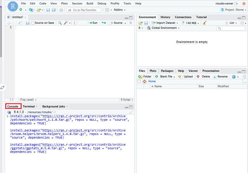
install.packages("https://cran.r-project.org/src/contrib/Archive/patchwork/patchwork_1.1.0.tar.gz", repos = NULL, type = "source", dependencies = TRUE)

install.packages("https://cran.r-project.org/src/contrib/Archive/broom.helpers/broom.helpers_1.4.0.tar.gz", repos = NULL, type = "source", dependencies = TRUE)

install.packages("https://cran.r-project.org/src/contrib/Archive/ggstats/ggstats_0.5.0.tar.gz", repos = NULL, type = "source", dependencies = TRUE)

Exercise: 练习：

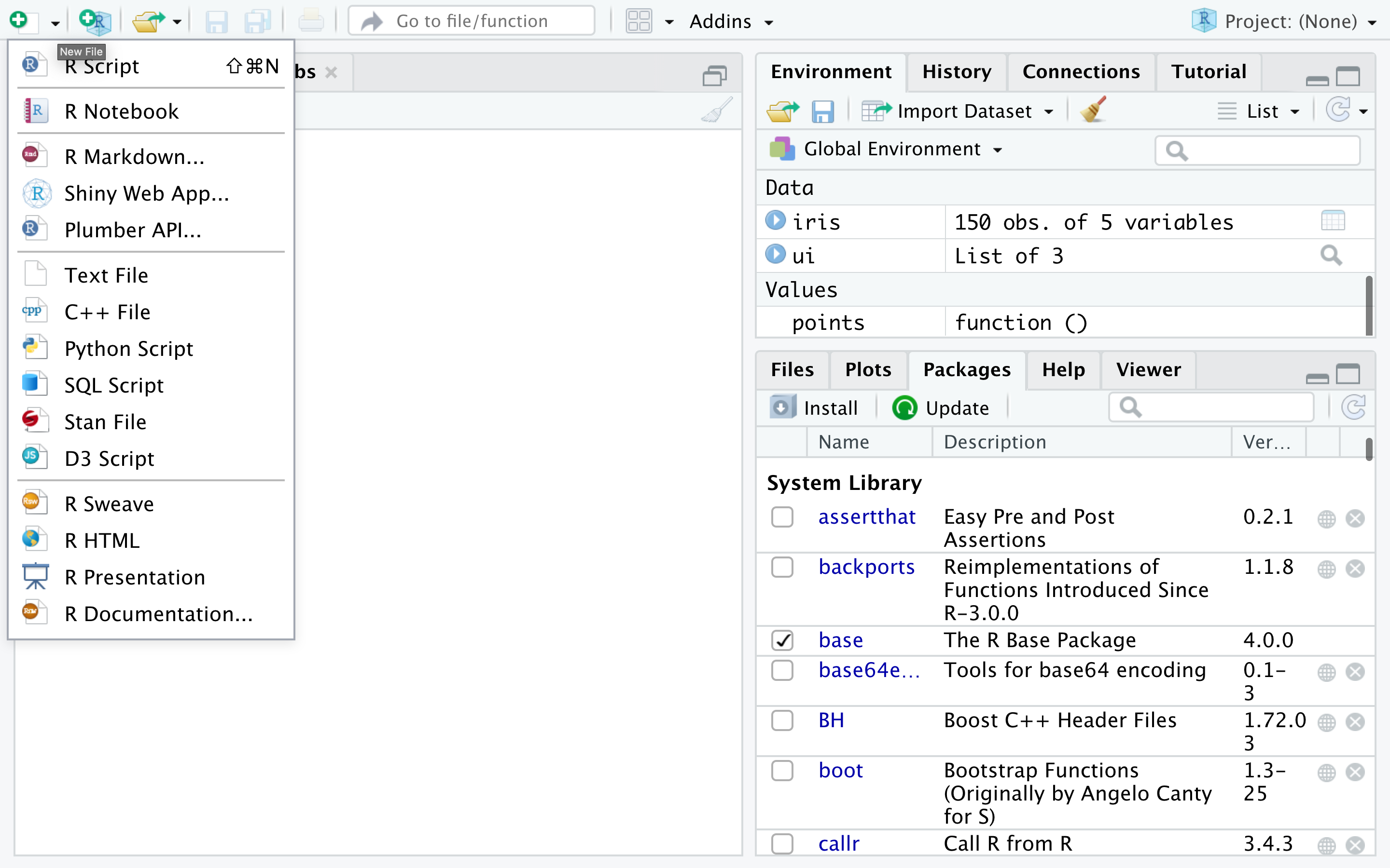
Click the plus symbol on the top left and click R Script to create a new R script, if you don't have one open already.
点击左上角的 plus 符号，然后点击 R Script 创建一个新的 R 脚本，如果你还没有一个打开的脚本的话。

You will use the iris dataset. If you don't have it loaded, copy and paste the following into your R script file.
您将使用鸢尾花数据集。如果您还没有加载它，请将以下内容复制并粘贴到您的 R 脚本文件中。
```
library(datasets)
data(iris)
```
In the previous lab, you installed the libraries necessary to create plots, let's execute the following commands:
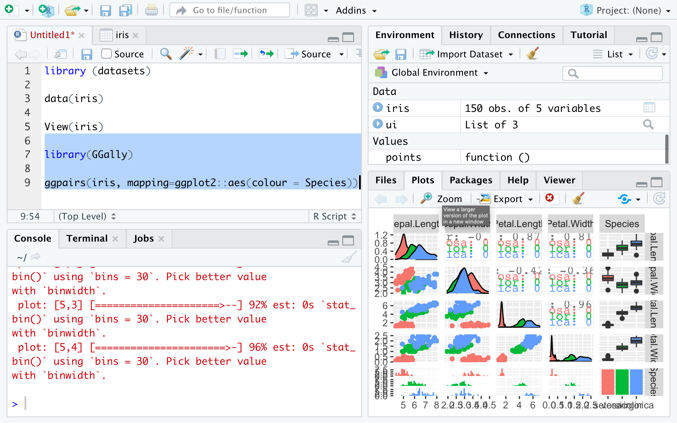
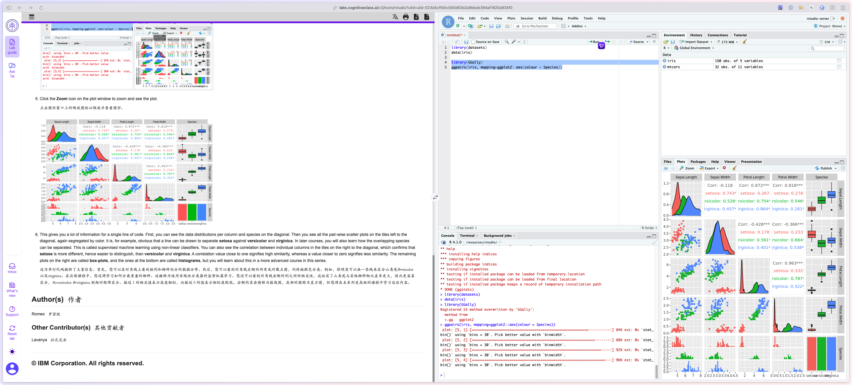
在上一节实验中，您安装了创建图形所需的库，让我们执行以下命令：
```
library(GGally)
ggpairs(iris, mapping=ggplot2::aes(colour = Species))
```
Select the commands and click Run on the top. You' ll see the following plot in the Plots window:
选中命令并在顶部点击 Run 。您将在图形窗口中看到以下图形：
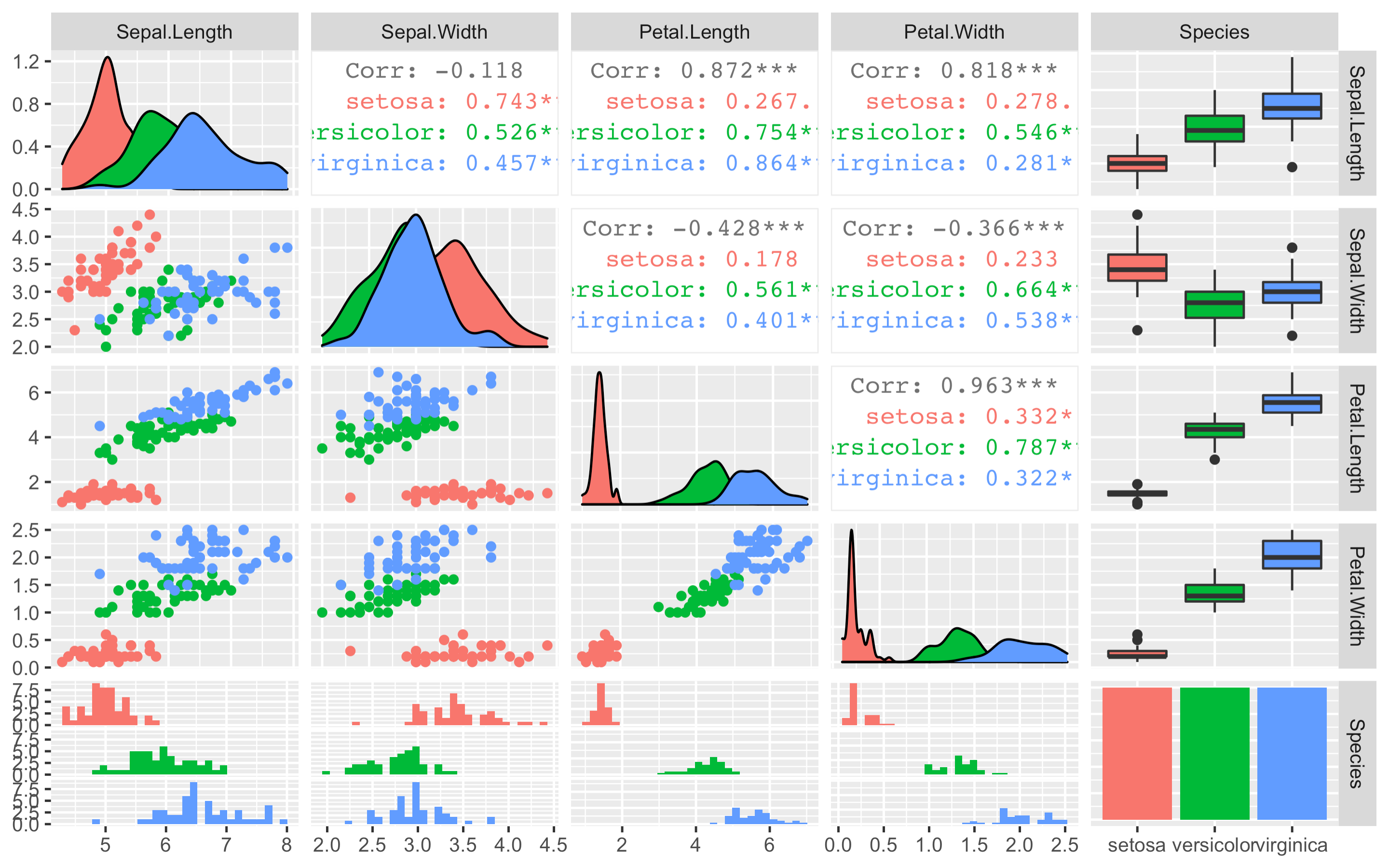
Click the Zoom icon on the plot window to zoom and see the plot.
点击图形窗口上的缩放图标以缩放并查看图形。
This gives you a lot of information for a single line of code. First, you can see the data distributions per column and species on the diagonal. Then you see all the pair-wise scatter plots on the tiles left to the diagonal, again segregated by color. It is, for example, obvious that a line can be drawn to separate setosa against versicolor and virginica. In later courses, you will also learn how the overlapping species can be separated. This is called supervised machine learning using non-linear classifiers. You can also see the correlation between individual columns in the tiles on the right to the diagonal, which confirms that setose is more different, hence easier to distinguish, than versicolor and virginica. A correlation value close to one signifies high similarity, whereas a value closer to zero signifies less similarity. The remaining plots on the right are called box-plots, and the ones at the bottom are called histograms, but you will learn about this in a more advanced course in this series.
这为单行代码提供了大量信息。首先，您可以在对角线上看到按列和物种划分的数据分布。然后，您可以看到对角线左侧的所有成对散点图，同样按颜色分类。例如，很明显可以画一条线来区分山鸢尾和versicolor 以及virginica。在后续课程中，您还将学习如何分离重叠的物种。这被称为使用非线性分类器的监督机器学习。您还可以看到对角线右侧的列之间的相关性，这证实了山鸢尾与其他物种相比差异更大，因此更容易区分，而versicolor 和virginica 则相对较难区分。接近 1 的相关值表示高度相似，而接近 0 的值表示相似度较低。右侧的其余图称为箱线图，底部的图称为直方图，但您将在本系列更高级的课程中学习这些内容。

Plotting with RStudio使用 RStudio 绘图

Author(s) 作者

Other Contributor(s) 其他贡献者

© IBM Corporation. All rights reserved.